Identify_aneuploid_cells_from_scRNAseq_data.Rmd

---
title: "Identify aneuploid cells from scRNAseq"
author: "Yiyun Lin"
date: '2024-05-21'
output:
  html_document: default
  pdf_document: default
---

```{r setup, include=FALSE}
knitr::opts_chunk$set(echo = TRUE)
```

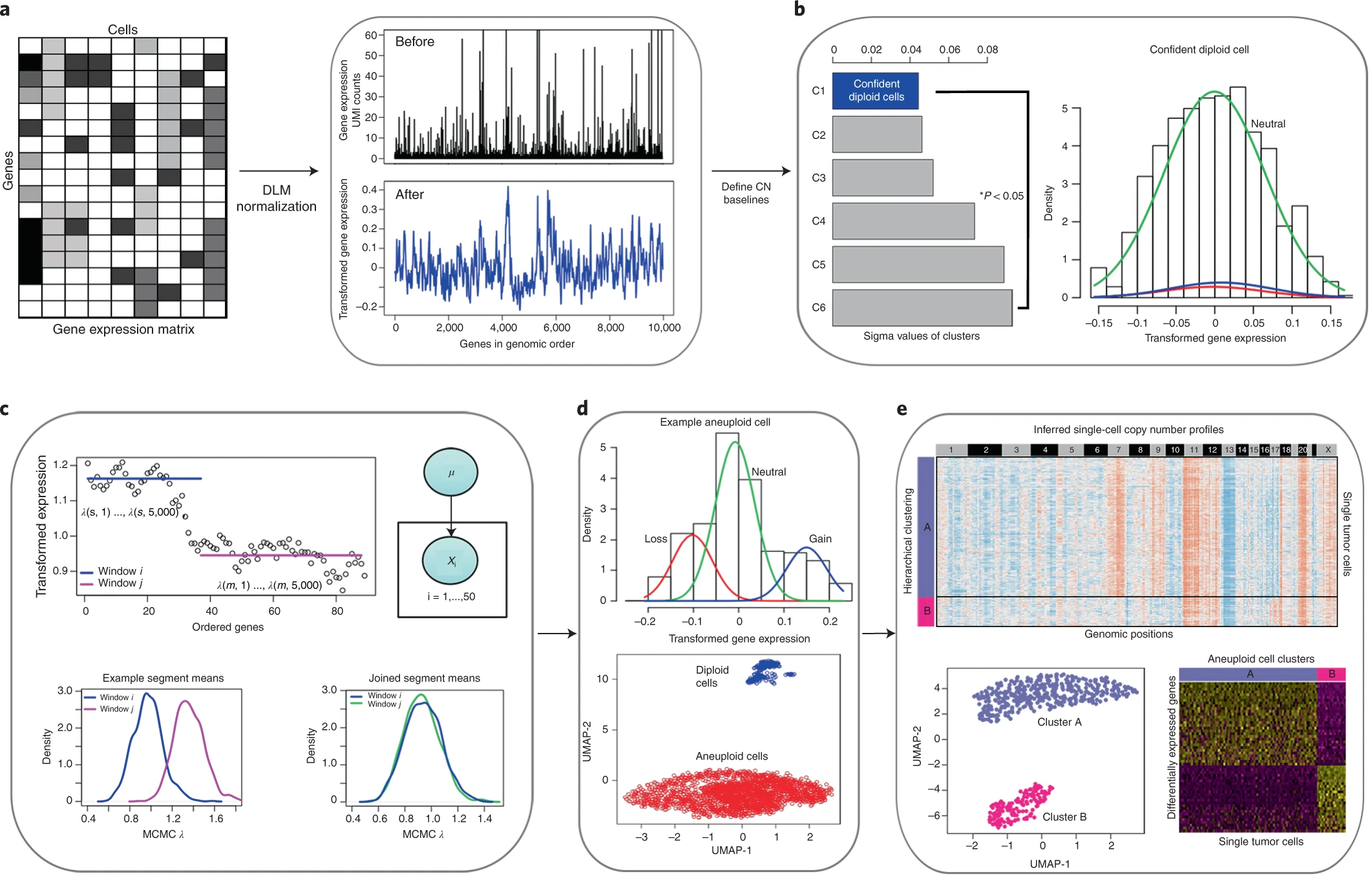
# Inference of genomic copy number variation from high-throughput single cell RNA sequencing data
A major challenge for single cell RNA sequencing of human tumors is to distinguish cancer cells from non-malignant cell types, as well as the presence of multiple tumor subclones. Previous studies showed many tumor cells are aneuploid with high extend of genomic alteration. CopyKAT and InferCNV are two computational tools to identify genome-wide copy number alterations in single cells to separate tumor cells from normal cells, and tumor subclones using high-throughput sc-RNAseq data. The underlying logic for calculating DNA copy number events from RNAseq data is that gene expression levels of many adjacent genes can provide depth information to infer genomic copy number in that region. Both tools will provide a copy number heatmap and aneuploid cell predictions in their results.


## Installation
Install copykat in R studio
```r
library("devtools")
install_github("navinlabcode/copykat")
```
Install inferCNV in R studio 
pre-requisite: Install the [JAGS](https://sourceforge.net/projects/mcmc-jags/files/JAGS/4.x/) package. This can be installed for Mac, Windows, or Linux. Be sure to download and install the corresponding package matching your OS.)

```r
library("devtools")
devtools::install_github("broadinstitute/infercnv")
```
<br />
<br />
<br />
<br />


## Overview of the CopyKAT analysis workflow.

__1.stabilize variance and smooth outliers:__\
The workflow takes the gene expression matrix of unique molecular identifier (UMI) counts as input for the calculations. The analysis begins with the annotation of genes in rows to order them by their genomic coordinates. Freeman–Tukey transformation11 is performed to stabilize variance, followed by polynomial dynamic linear modeling (DLM)12 to smooth the outliers in the single-cell UMI counts (Fig. 1a).

__2.identify the confident normal cells:__\
The next step is to detect a subset of diploid cells with high confidence to infer the copy number baseline values of the normal 2N cells. To do this, we pool single cells into several small hierarchical clusters(hclust) and estimate the variance of each cluster using a Gaussian mixture model (GMM). The cluster with minimal estimated variance is defined as the ‘confident diploid cells’ by following a strict classification criterion (Fig. 1b left panel). A single cell is  defined as a confident diploid cell when the neutral distribution account for at least 99% of the expressed genes (Fig. 1b right panel).

__3.identify the breakpoints and calculate the ratio in segments:__\
To detect chromosome breakpoints, we integrate a Poisson-gamma model and Markov chain Monte Carlo (MCMC) iterations to generate posterior means per gene window(take at least 25 genes per segment) and then apply Kolmogorov–Smirnov (KS) tests to join adjacent windows that do not have significant differences in their means(merge when D< KS.cut). After identify the breakpoints across genome, the final copy number values for each segment are then calculated as the posterior averages of all genes spanning across the adjacent chromosome breakpoints in each cell (Fig. 1c).

__4.identify the aneuploid and diploid cells:__\
We then perform hierarchical clustering of the single-cell copy number data, and cutree 2 to identify the largest distance between the aneuploid tumor cells and the diploid stromal cells; The clsuter with the most overlap of pre-defined confident normal will be classified as diploid cells. however, if the genomic distance is not significant, we switch to the GMM definition model to predict single tumor cells one by one (Fig. 1d).

__5.identify subclone structure:__\
Finally, we cluster the single-cell copy number data to identify clonal subpopulations and calculate consensus profiles representing the subclonal genotypes for further analysis of their gene expression differences (Fig. 1e).

![Copykat workflow.](https://media.springernature.com/full/springer-static/image/art%3A10.1038%2Fs41587-020-00795-2/MediaObjects/41587_2020_795_Fig1_HTML.png?as=webp)

<br />
<br />
<br />
<br />


## Running copykat
### step 1: prepare the readcount input file
The only input file that you need to prepare to run copykat is the raw gene expression matrix, with gene ids in rows and cell names in columns. The gene ids can be gene symbol or ensemble id. The matrix values are often the count of unique molecular identifier (UMI) from nowadays high througput single cell RNAseq data. The early generation of scRNAseq data may be summarized as TPM values or total read counts, which should also work. 

option1.prepare from 10X output.
```r
# data was from TNBC5 in Ruli Gao et al, NBT, 2021 
data.path.to.cellranger.outs <-"/volumes/seq/projects/ARTEMIS/cellranger_v3_10/ART89PreTX_C/outs/filtered_feature_bc_matrix/"
library(Seurat)
library(readr)
library(dplyr)
raw <- Read10X(data.dir = data.path.to.cellranger.outs)
raw <- CreateSeuratObject(counts = raw, project = "copycat.test", min.cells = 0, min.features = 0)
exp.rawdata <- as.matrix(raw@assays$RNA@counts)
exp.rawdata[1:5,1:5] #rownames: gene symbol; colnames: cell id
```
option2.prepare from processed seurat obejct.
```r
raw = read_rds('/volumes/USR1/yiyun/Project/CSHL_workshop/input/input_seu.rds')
library(Seurat)
exp.rawdata <- as.matrix(raw@assays$RNA@counts)
raw@meta.data$celltype %>% table()
normal = rownames(raw@meta.data[raw@meta.data$celltype %in% c('Fibro', 'Mye', 'T'),]) #copykat can also take normal stromal cellname as reference
```

### step 2: run copykat
Now we have prepared the input (raw UMI count matrix). we are ready to run copykat.\
__parameters:__\
__id.type = 'S'__ (input matrix gene_id is gene symbol);\
__ngene.chr = 5__ (cell filter: at least 5 genes in each chromosome to calculate DNA copy numbers, to keep more cells, we can tune this down to ngene.chr=1)\
__win.size = 25__ (gene window: 25 genes per window)\
__LOW.DR = 0.05__, __UP.DR__=0.2 (gene filter: keep genes expressed in >5%(LOW.DR) cells for data quality control. use gene expressed in >20%(UP.DR) cells for segmentation)\
__sam.name = "test"__ (your sample name)\
__distance = "euclidean"__ (distance parameters for clustering that include "euclidean" distance and correlational distance, ie. 1-"pearson" and "spearman" similarity. In general, corretional distances tend to favor noisy data, while euclidean distance tends to favor data with larger CN segments.)\
__norm.cell.names = "" __ (if you already identify the stromal cells such as fribroblast, meyloids, t cell, endothelial cells, you can output the cell anmes in the matrix to tell copykat here we have a reference data, you can use to calculate the baseline ratio. Default is "", meaning NOT input any normal reference)\
__output.seg = "FALSE"__ (output seg file which can be directly loaded to IGV viewer for visualization. Default is FALSE)\
__plot.genes = "TRUE"__ (plot of single cell copy number results, using gene by cell matrix. This is by default, plot.genes="TRUE". Gene names are labelled at the bottom of heatmap. Need to zoom in to read the tiny fonts)\
__genome = "hg20"__ (the input data genome annotation version, if it's a mouse data, use "mm10")\
__n.cores=20__ (parallel computation)\

```r
library(copykat)
#with ref
copykat.test <- copykat(rawmat=exp.rawdata, id.type="S", ngene.chr=5, win.size=25, KS.cut=0.1, LOW.DR=0.05, UP.DR=0.2, sam.name="test", distance="euclidean", norm.cell.names=normal, output.seg="FLASE", plot.genes="TRUE", genome="hg20",n.cores=20)

#without ref
copykat.test <- copykat(rawmat=exp.rawdata, id.type="S", ngene.chr=5, win.size=25, KS.cut=0.1, LOW.DR=0.05, UP.DR=0.2, sam.name="test", distance="euclidean", norm.cell.names="", output.seg="FLASE", plot.genes="TRUE", genome="hg20",n.cores=20)
```

### step 3: read copykat results

```r
setwd('/volumes/USR1/yiyun/Project/CSHL_workshop/output_copykat_noref_normal/')
library(Seurat)
library(readr)
library(dplyr)

pred.test <- read.table('./test_copykat_prediction.txt',header = T)
head(pred.test)
# 1989 aneuploid cells (some cells were classified as not defined because of low quality)
table(pred.test$copykat.pred) 
pred.test <- pred.test[-which(pred.test$copykat.pred=="not.defined"),] 
head(pred.test)

raw = readRDS('/volumes/USR1/yiyun/Project/CSHL_workshop/input/input_seu.rds')
raw$celltype %>% table() 

CNA.test <- read.table('./test_copykat_CNA_results.txt',header = T)
CNA.test[1:5,1:5]
dim(CNA.test)
```

### step 4: input copykat ratio matrix to copykit for further analysis
```r
source('/volumes/USR1/yiyun/Project/CSHL_workshop/Copykit_copykat_functions.R')
library(copykit, lib.loc = "/opt/R/4.1.2/lib/R/library")

cpkobj <- Copykit_copykat(CNA_result = CNA.test, genome_version = 'hg19',resolution = '200k',method = 'copykat')
assay(cpkobj, "segratio_unlog") <- 2^assay(cpkobj, "segment_ratios")
assay(cpkobj, "logr") <- assay(cpkobj, "segment_ratios")

meta <- colData(cpkobj) %>% data.frame()
  
#add copykat annotation
meta <- left_join(meta,pred.test)
colData(cpkobj)$copykat.pred = meta$copykat.pred
#add celltype annotation
cell_anno <- read.table('/volumes/USR1/yiyun/Project/CSHL_workshop/input/input_cell_annotation.txt') %>% set_colnames(c('cell.names','cell.types'))
meta <- left_join(meta,cell_anno)
colData(cpkobj)$cell.types = meta$cell.types
  
color_heat = circlize::colorRamp2(breaks = c(-0.5,0,0.5), c("dodgerblue3", "white", "firebrick3"))
pdf('heatmap_celltype.pdf',width = 10,height = 10)
print(plotHeatmap_copykatST(cpkobj,n_threads = 30, pt.name = 'test', order_cells = "hclust",
                        use_raster = T, assay = "segratio_unlog", col = color_heat,
                        row_split = 'cell.types',
                        label = c('copykat.pred','cell.types')))
dev.off()
```
![copykat heatmap annotated with cell type.](/volumes/USR1/yiyun/Project/CSHL_workshop/output_copykat_noref_normal/heatmap_celltype.png){width=65%}.


### step 5: clustering to identify subclones
```r
tumor <- cpkobj[, colData(cpkobj)$copykat.pred == 'aneuploid']
tumor <- runUmap(tumor, n_neighbors = 30, min_dist = 0)

seg_data <- t(SummarizedExperiment::assay(tumor, 'segment_ratios'))
seg_data[1:5,1:5]  
hcl <- hclust(parallelDist::parDist(as.matrix(seg_data),threads =30, method = "euclidean"), method = "ward.D2")
k <- 10
tree <- cutree(hcl,k=k)
meta <- colData(tumor)
df <- cbind(tree, meta$sample) %>% data.frame()%>% set_colnames(c(paste0('hclust_',k),'sample'))
df[,paste0('hclust_',k)] = factor(df[,paste0('hclust_',k)],levels = as.character(unique(df[,paste0('hclust_',k)])))
table(df$hclust_10)
SummarizedExperiment::colData(tumor) <- cbind(SummarizedExperiment::colData(tumor),df%>% dplyr::select(-sample))
  
pdf('heatmap_tumor_subclones.pdf',width = 10,height = 10)
print(plotHeatmap_copykatST(tumor,n_threads = 30, pt.name = 'test', order_cells = "hclust",
                              use_raster = T, assay = "segratio_unlog", col = color_heat,
                              row_split = 'hclust_10',
                              label = c('hclust_10','cell.types')))
dev.off()
```
![copykat heatmap annotated with subclones.](/volumes/USR1/yiyun/Project/CSHL_workshop/output_copykat_noref_normal/heatmap_tumor_subclones.png){width=65%}.

### step 6: comparing the result with ground truth
copykat not captured:					
chr2q gain,	chr3p loss,	chr4 loss,	chr6 loss,	chr18 loss,	chrX gain & chrX loss
![check results with ground truth](/volumes/USR1/yiyun/Project/CSHL_workshop/output_copykat_noref_normal/comparing_GT.png)
<br />
<br />
<br />
<br />

## Running inferCNV
### step 1: prepare inferCNV input file
```r
raw = read_rds('/volumes/USR1/yiyun/Project/CSHL_workshop/input/input_seu.rds')
library(Seurat)
library(readr)
library(dplyr)

#count matrix
exp.rawdata <- as.matrix(raw@assays$RNA@counts)
write.table(exp.rawdata,'/volumes/USR1/yiyun/Project/CSHL_workshop/input/input_count_matrix.txt',row.names = T,quote = F,sep = '\t')

#cell type annotation dataframe
anno = raw@meta.data %>% select(cellname, celltype)
colnames(anno) = NULL
write.table(anno,'/volumes/USR1/yiyun/Project/CSHL_workshop/input/input_cell_annotation.txt',row.names = F,quote = F,sep = '\t')
  
gene chromosomal position annotation dataframe
full.anno <- read.delim("/volumes/USR1/yiyun/Project/CSHL_workshop/input/gencode.hg38.v28.annotation.abs.band.bed", header = TRUE, stringsAsFactors=FALSE)
gene_anno = full.anno %>% 
    select(hgnc_symbol,chromosome_name,start_position, end_position) %>% 
    filter(hgnc_symbol %in% rownames(exp.rawdata)) %>% 
    filter(!duplicated(hgnc_symbol))
rownames(gene_anno) = gene_anno$hgnc_symbol
gene_anno = gene_anno %>% select(hgnc_symbol,chromosome_name,start_position,end_position)
gene_anno$chromosome_name = paste0('chr',gene_anno$chromosome_name)
colnames(gene_anno) = NULL
write.table(gene_anno,'/volumes/USR1/yiyun/Project/CSHL_workshop/input/input_gene_annotation.txt',row.names = F,quote = F,sep = '\t')
```

### step 2: Creating an InferCNV object based on inputs
```r
#with ref
infercnv_obj = CreateInfercnvObject(raw_counts_matrix= './input_count_matrix.txt',
                                      annotations_file="./input_cell_annotation.txt",
                                      delim="\t",
                                      gene_order_file="./input_gene_annotation.txt",
                                      ref_group_names=c('Fibro', 'Mye', 'T'))
#without ref
infercnv_obj = CreateInfercnvObject(raw_counts_matrix= './input_count_matrix.txt',
                                      annotations_file="./input_cell_annotation.txt",
                                      delim="\t",
                                      gene_order_file="./input_gene_annotation.txt",
                                      ref_group_names=NULL)
```   

### step3: After creating the infercnv_obj, you can then run the standard infercnv procedure via the built-in 'infercnv::run()' function
```r
infercnv_obj = infercnv::run(infercnv_obj,
                               cutoff=0.1,  # use 1 for smart-seq, 0.1 for 10x-genomics
                               out_dir="/volumes/USR1/yiyun/Project/CSHL_workshop/output_infercnv_ref_normal/",  # dir is auto-created for storing outputs
                               cluster_by_groups=T,   # cluster
                               denoise=T,
                               num_threads = 20,
                               HMM=T)
```        

### step4: read inferCNV results
```r
library(readr)
library(dplyr)
library(inferCNV)
library(Seurat)
setwd('/volumes/USR1/yiyun/Project/CSHL_workshop/output_infercnv_ref_normal/')
infercnv_obj <- readRDS('./preliminary.infercnv_obj')
  
# 'infercnv_obj@ expr.data' : contains the processed expression matrix as it exists at the end of that stage for which that inferCNV object represents.
infercnv_obj@ expr.data[1:5,1:5]
# 'infercnv_obj@reference_grouped_cell_indices' : list containing the expression matrix column indices that correspond to each of the normal (reference) cell types.
lapply(infercnv_obj@reference_grouped_cell_indices, head)
# 'infercnv_obj@observation_grouped_cell_indices' : similar list as above, but corresponds to the tumor cell types.
lapply(infercnv_obj@observation_grouped_cell_indices, head)

#check the aneuploid cell prediction:
subclone <- read.table('/volumes/USR1/yiyun/Project/CSHL_workshop/output_infercnv_noref_normal/infercnv.observation_groupings.txt')
head(subclone)
nrow(subclone) 

#nrow(subclone) match to the number of Tumor cells previous annotated.
raw = readRDS('/volumes/USR1/yiyun/Project/CSHL_workshop/input/input_seu.rds')
raw$celltype %>% table()

subclone$Dendrogram.Group %>% table() # the number of subclone identified by inferCNV
```  
![inferCNV heatmap annotated with subclones.](/volumes/USR1/yiyun/Project/CSHL_workshop/output_infercnv_noref_normal/infercnv.png){width=65%}.

### step 5: comparing the result with ground truth
inferCNV not captured:					
chr2q gain,	chr3p loss,	chr4 loss,	chr6 loss, chr10 loss, chr11 loss, chr18 loss,	chrX gain & chrX loss
![check results with ground truth](/volumes/USR1/yiyun/Project/CSHL_workshop/output_infercnv_noref_normal/comparing_GT.png)

<br />
<br />
<br />
<br />

## Comparison between copykat and inferCNV
### running time: 
inferCNV: 3 hours (using 20 cores)\
copykat: 1 hour (using 20 cores)\

### result format:
inferCNV: normalized genes epxression matrix, ordered by chromosome position\
copykat: copy number ratios in 220k genomic bin, easily take by copykit\

### plot
inferCNV:fail to capture chr10 & chr11 loss comparing to copykat
![copykat and inferCNV comparison](/volumes/USR1/yiyun/Project/CSHL_workshop/copykat_inferCNV.png)